Tech Tip Tuesday: How Do You Split Up First and Last Names In An Excel Sheet?

Sometimes you need to use data from Excel in other software programs. To do so, you may need to format the data for it to transfer properly. In this case, we’re going to split up first and last names in one column into two separate columns.

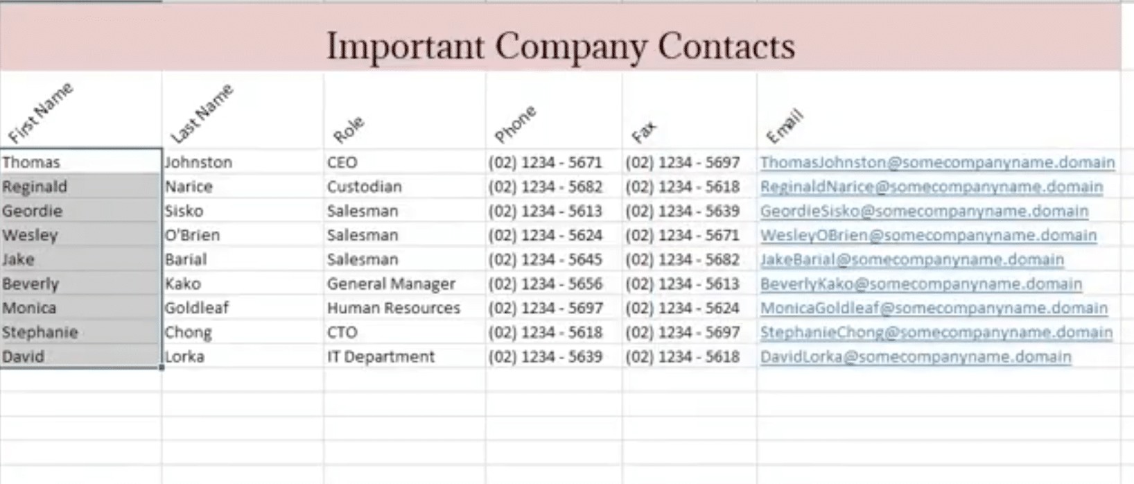
Here, we have our company directory in Excel. You can see that the Name Column contains both the first and last names of our employees. We want to change this so the first name is in one column and the last name is in the column next to it.

Instead of doing this manually by copy and pasting as some people would do, we’ll show you an easier way to do this.

1. Start by inserting a new column next to the Name Column.

2. Rename your column headings to First Name and Last Name.

3. Select all the names in the First Name column.

4. From the top ribbon, go to the Data Tab and click “Text To Columns.”

This opens Excel’s “Text To Columns” Window.

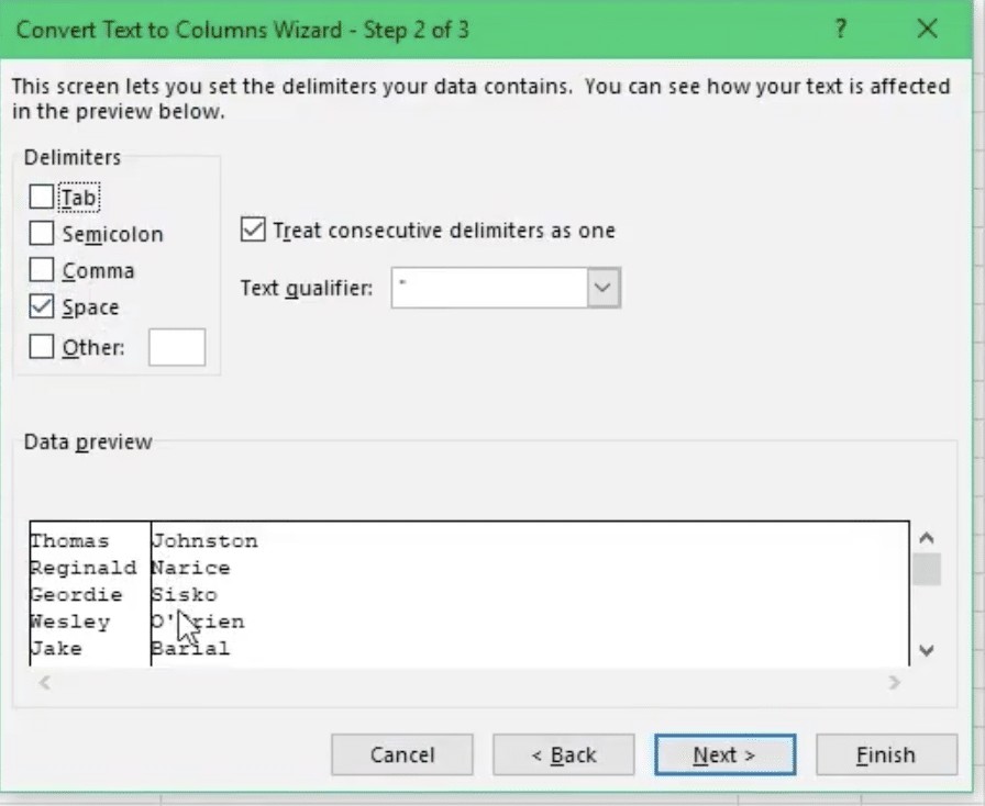
5. Select the datatype as “Delimited.”

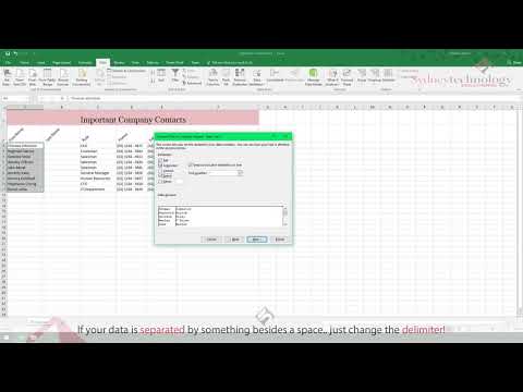
6. Next, select the appropriate Delimiter to split the names. Because we have a space after the first name, we’re going to choose the “Space” Delimiter.

7. The next step offers you more advanced options that you can choose from.

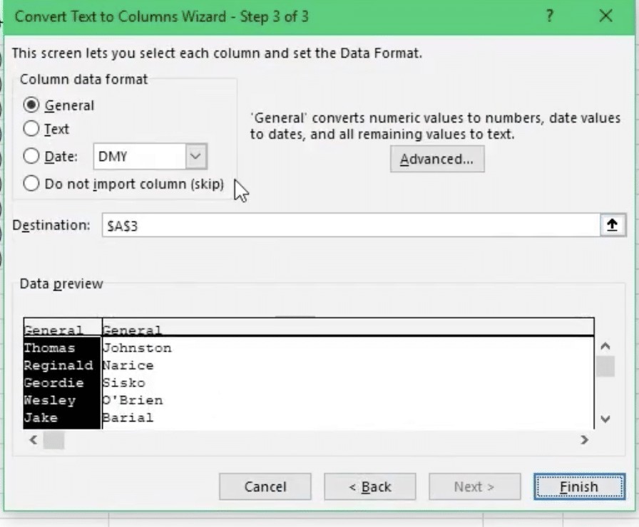
8. For our purpose, we don’t need to choose any other options. So, just click “Finish” and you’ll see your first and last names split into two columns.

You can use this process to separate all kinds of text columns in Excel with any kind of data. Hope this helps!

Bonus! 10 Handy Quick Excel Tips For You

1. Organisation Tip

Note: Be sure to keep all values separate and in their own cells. Never put them in formulas. The Excel VALUE function can be used to convert a text value that represents a number to the actual number.

When you make changes to your formula, and you include values, it will present complexities. Instead, you should use formulas that link to and reference cells.

2. Column Width Solution

Click on the column that you need to change and alter the width from the pop-up. Or you can simply DOUBLE CLICK the column and drag the right corner of it to the width you prefer.

3. How To Anchor Values In A Formula

Let’s say you have columns specifying ACCOUNT, UNITS SOLD, REVENUE and you want to designate a formula for Price multiplied by Units Sold.

• Select the REVENUE column. (Be sure to clean out any data.)
• Go to NO FILL>NO BORDERS
• Click on the cell you want to be the Anchor. Hit F4.
• This cell will now always be the anchor for your formula.

4. Did You Know That You Can Automatically Populate Cells With Formulas?

Drag the bottom right of the formula cell to the cells you want to populate. Double Click and it will populate all the cells with the formula data. So easy!

5. A Few Quick Navigation Shortcuts

Let’s say that you have a spreadsheet with hundreds of lines of data. How are you going to highlight all these cells? You can’t drag all the way to the bottom. Here’s how:

• Click CONTROL and hit the ARROW DOWN button. This will send you to the bottom of the worksheet.
• If you want to go up to the top, hit CONTROL and ARROW UP.
• To go back and forth between the top and bottom, use CONTROL>PERIOD.

6. Sum It Up

If you use the typical cell + cell + this can be tedious and time-consuming. Try using

EQUAL SUM. Type SUM into the cell and drag the data you want to the SUM cell. It will calculate the sum automatically!

You can also use AUTO SUM in the top ribbon. Place your mouse symbol below the data and click ENTER. Your sum will magically appear.

7.How To Reveal Data That’s Hidden

Select all the cells that contain the hidden data. Go to the top ribbon and select WRAP TEXT. Use the NAVIGATION WINDOW to reveal your data.

• COPY values >PASTE SPECIAL and paste the VALUE, or10. Copy Text Quickly

8. How To Enter Text Quickly

Enter the text that you want, (e.g. “January”) and DOUBLE CLICK it, and Excel will figure out how to populate cells with the remaining months! Excel’s pretty smart!

9. Enter Different (Un-Identical) Information Into Non-Adjacent Cells

Choose and select which cells you want the data to appear in. Select CONTROL+Enter the number of items you want, and all the selected cells will populate with data.

10. How To Easily Date Your Work

Select the cell you want to enter the date in.

Click = TODAY and today’s date will magically appear!

If You Liked This Information, Be Sure To Check Out Some Of Our Blogs!

Microsoft Excel & Power BI

Resolving Complexity: Office 365 Updates That Are Taking User Experience To New Heights

The Business Owner’s Guide To Microsoft Office 365